2.1 Sequencing QC
Teaching: 90 min || Exercises: 30 min
Overview
2.1.1 Background
Before we delve into having a look at our own genomic data. Lets take some minutes to explore what to look out for when performing Quality Control (QC) checks on our sequences. For this part of the course, we will largely focus on third generation sequences obtained from ONT sequencers. As you may already know from our previous lesson, the main output files expected from our ONT sequencer are .fast5 files which are readily converted to FastQ files for downstream analysis. Here, we will attempt to quality trim our Nanopore data using PoreChop and/or fastp and assess basic sequencing QC utilizing NanoPlot, fastq-scan and FastQC. Other frequently used QC tools include PycoQC. We would then check for contamination using both GC content statistics and Kraken 2. We will also combine reports from all these tools using MultiQC.
2.1.2 Joining multiple FastQ files
Normally, Guppy barcoder writes demultiplexed reads to multiple FastQ files per barcode, each having (normally) 4000 reads. To go further with your sequence data, you will have to join these FastQ files together into a single file per barcode.
We can do this in two ways with simple lines of commands.
-1 Unzip gunzip the files, combine them into one zipped file gzip and redirect it > into the required file name.
The basic command looks like this.
gunzip -c *.fastq.gz | gzip -c > joined.fastq.gzYou can now run the command on your first set of fastq files.
gunzip -c *.fastq.gz | gzip -c > barcode30.fastq.gzThis uses a lot of memory and may not be the best option to perforn this task.
-2 The second way to do this is to concatenate the files using the cat command.
cat *.fastq.gz > barcode30.fastq.gzLet’s navigate into any of our ONT sequence directory and run any of the above codes. For instance let’s run the command on barcode30. Navigate to the barcode30 directory, copy paste the command and run it.
QC assessment of ONT data
As you may already know, QC is an important part of any analysis. In this section we are going to look at some of the metrics and graphs that can be used to assess the QC of NGS data.
Base quality
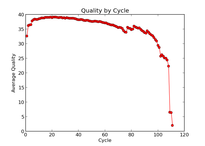
Illumina sequencing technology relies on sequencing by synthesis. One of the most common problems with this is dephasing. For each sequencing cycle, there is a possibility that the replication machinery slips and either incorporates more than one nucleotide or perhaps misses to incorporate one at all. The more cycles that are run (i.e. the longer the read length gets), the greater the accumulation of these types of errors gets. This leads to a heterogeneous population in the cluster, and a decreased signal purity, which in turn reduces the precision of the base calling. The figure below shows an example of this.
Because of dephasing, it is possible to have high-quality data at the beginning of the read but really low-quality data towards the end of the read. In those cases you can decide to trim off the low-quality reads, for example using a tool called Trimmomatic. In this workshop, we will do this using the tool fastp. In addition to trimming low quality reads, fastpwill also be used to trim off Illumina adapter/primer sequences.
The figures below shows an example of a high-quality read data (left) and a poor quality read data (right).
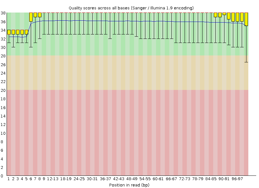
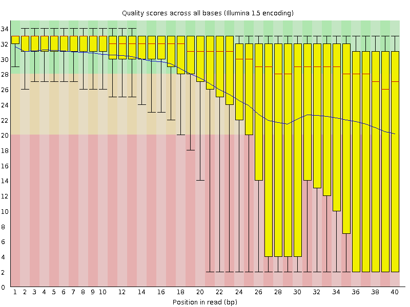
Base Quality Comparison
In addition to Phasing noise and signal decay resulting from dephasing issues described above, there are several different reasons for a base to be called incorrectly. You can lookup these later by clicking here.
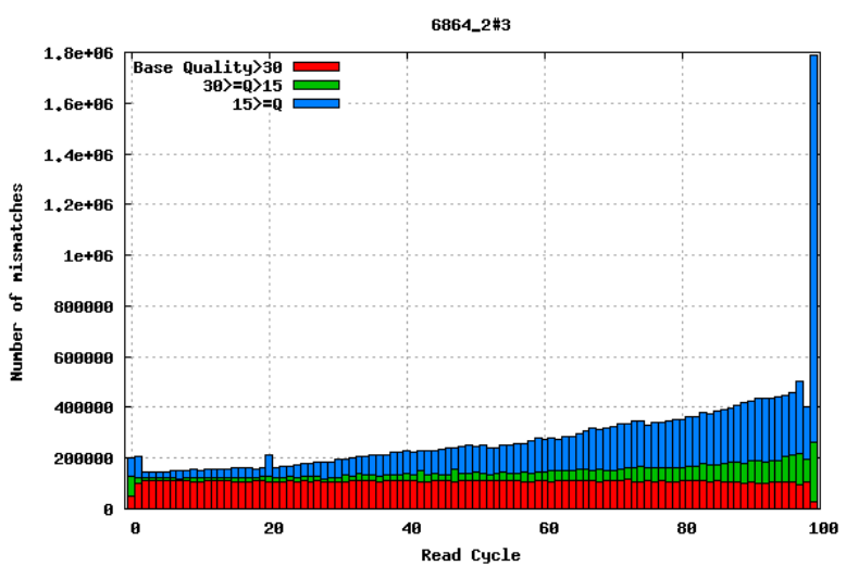
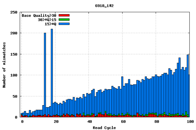
Mismatches per cycle
Aligning reads to a high-quality reference genome can provide insight to the quality of a sequencing run by showing you the mismatches to the reference sequence. This can help you detect cycle-specific errors. Mismatches can occur due to two main causes, sequencing errors and differences between your sample and the reference genome, which is important to bear in mind when interpreting mismatch graphs. The figures below show an example of a good run (top) and a bad one (bottom). In the first figure, the distribution of the number of mismatches is even between the cycles, which is what we would expect from a good run. However, in the second figure, two cycles stand out with a lot of mismatches compared to the other cycles.
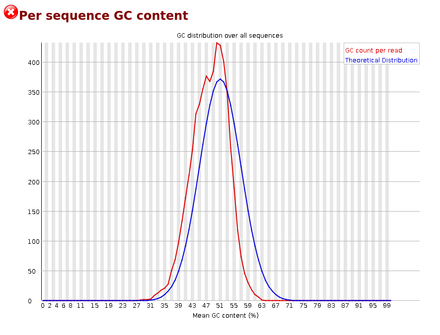
GC bias
It is a good idea to compare the GC content of the reads against the expected distribution in a reference sequence. The GC content varies between species, so a shift in GC content like the one seen below (right image) could be an indication of sample contamination. In the left image below, we can see that the GC content of the sample is about the same as for the theoretical reference, at ~65%. However, in the right figure, the GC content of the sample shows two distribution, one is closer to 40% and the other closer to 65%, indicating that there is an issue with this sample — a possible missed sample. Note that, suspecting contamination is perfectly fine for the species we are dealing with (MTBC). For other bacteria where there may be possibility of gene transfer, one can imagine that, such a situation may be from inheriting some plasmids that have a totally different GC content to the bacteria chromosome (This is arguable though).
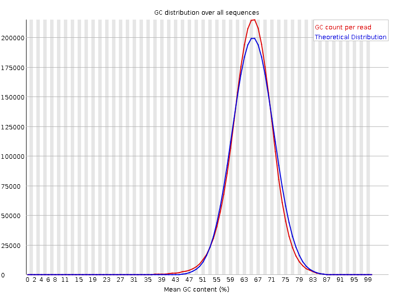
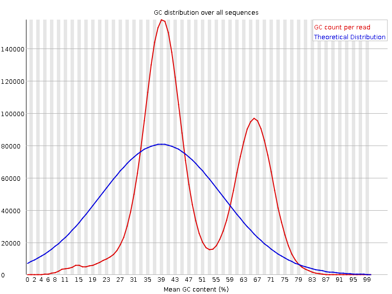
Figure: Base Quality Comparison
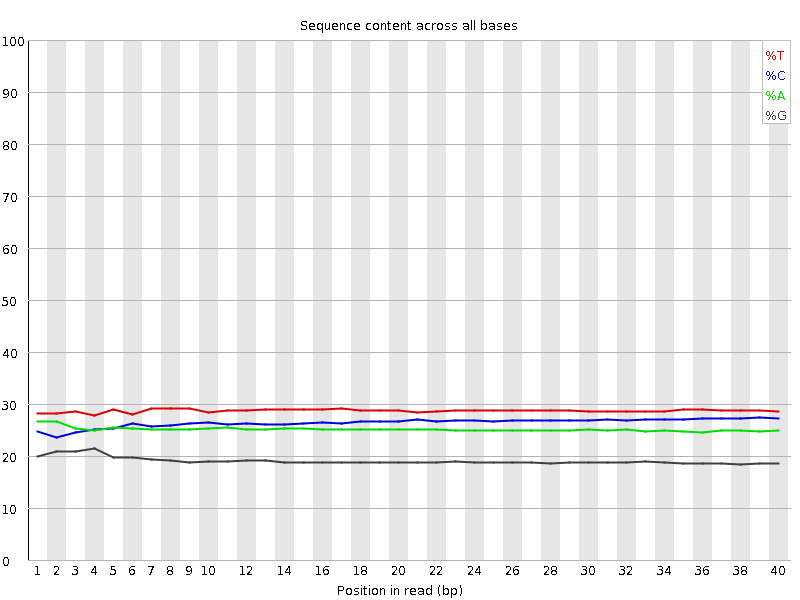
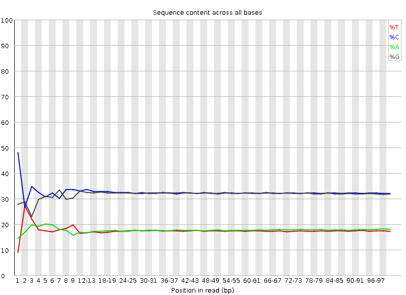
GC content by cycle
Looking at the GC content per cycle can help detect if the adapter sequence was trimmed. For a random library, it is expected to be little to no difference between the different bases of a sequence run, so the lines in this plot should be parallel with each other like in the first of the two figures below. In the second of the figures, the initial spikes are likely due to adapter sequences that have not been removed.
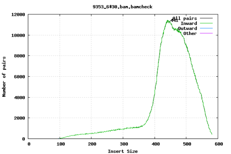
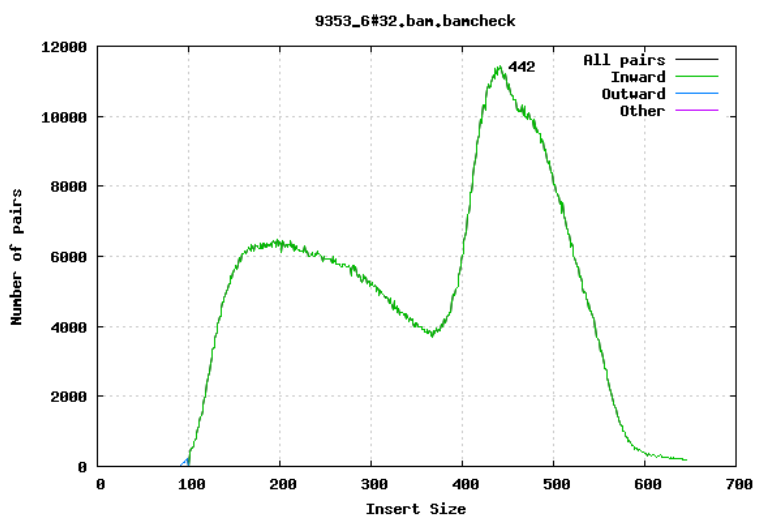
Insert size
For paired-end sequencing the size of DNA fragments also matters. In the first of the examples below, the insert size peaks around 440 bp. In the second however, there is also a peak at around 200 bp. This indicates that there was an issue with the fragment size selection during library prep.
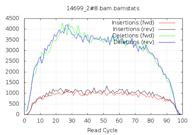
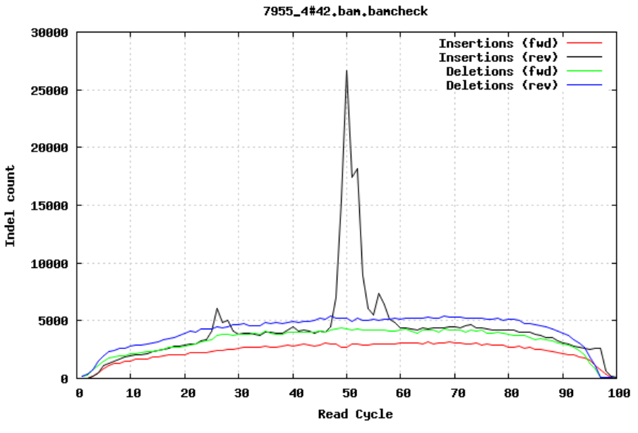
Insertions/Deletions per cycle
Sometimes, air bubbles occur in the flow cell, which can manifest as false indels. The spike in the second image provides an example of how this can look.
In addition to the QC plots you’ve encountered so far, there are other metrics that are generated with very powerful tools. For this workshop, we will explore these quality metrics with the help of fastq-scan and FastQC tools. It is often not a good practice to carry on analysis on samples that are contaminated with sequences from other species. We will identify contamination using either one of two ways. As earlier mentioned, the GC content varies between species, so a shift in GC content could be an indication of sample contamination. One other way of identifying sample contamination is by using specialized tools to determine/predict the species composition of your sample. For this course, we will determine species composition using the Kraken 2 database.
2.1.4 Generating QC stats and metrics
We are now ready to explore some quality metrics on our Nanopore sequence data.
This tutorial uses NanoPlot, fastq-scan, FastQC, fastp, PoreChop, Kraken 2, Bracken and MultiQC, which have been preinstalled for you in a virtual environment called qc_ont. This is to help speed up the pace of the workshop. However, NanoPlot is in a seperate environment due to dependency issues.
If for some reason, this environment is not pre-created for you, you can refer to the page for creating this conda environment. This will also be a good practice for you. In a latter chapter of the course, you will also be introduced to how to set up these virtual environments and explore its usefulness. For each tool, to get help messages that describe how they are used, you can simply type the name of the tool and hit enter. This only works if you activate the environment in which the tools have already been installed. Alternatively, you can use the help flag
-help or -h as appropriate. You can also invoke the manual of any tool (where available) by using the man command followed by the name of the tool.
Disk Usage I — Before analysis
Before we start investigating our genomic sequences, let’s pause and check the space of our current working directory.
You can do this with the disk usage du command
du -hCurrent Disk Space In QC Directory
~497MNow, keep this value in mind, we will come back to it at the end of the chapter.
NanoPlot
Nanoplot is a plotting tool for long read sequencing data and alignments. It is also available as a web service.
In addition to various plots also a NanoStats file is created summarizing key features of the dataset.
This script performs data extraction from Oxford Nanopore sequencing data in the following formats:
- fastq files (can be bgzip, bzip2 or gzip compressed)
- fastq files generated by albacore, guppy or MinKNOW containing additional information (can be bgzip, bzip2 or gzip compressed)
- sorted bam files
- sequencing_summary.txt output table generated by albacore, guppy or MinKnow basecalling (can be gzip, bz2, zip and xz compressed)
- fasta files (can be bgzip, bzip2 or gzip compressed) Multiple files of the same type can be offered simultaneously
Now run Nanoplot on your sample and interpret the html file produced.
NanoPlot -t 2 --fastq barcode30.fastq.gz --maxlength 40000 --plots dot --legacy hexNow that we are done with NanoPlot, let’s deactivate the nanoplot environment and go ahead and activate the qc_ont environment, so we can run the remaining tools:
mamba deactivatemamba activate qc_ontfastq-scan
fastq-scan is a very quick tool that reads a FASTQ from STDIN and outputs summary statistics (read lengths, per-read qualities, per-base qualities) in JSON format.
You can now go ahead and perform the fastq-scan with the below command.
Try this command out first. You may have to add < after the zcat command depending on your OS. zcat works differently with different OS.
Do this to run any of the ONT data and report on your findings:
zcat barcode30.fastq.gz | fastq-scan -g 4000000 > barcode30_fastq-scan.json*NB. In the above command, we assume a genome size of 4Mb.
You should now see one new file generated in your current directory.
To see if the file have been created, use this command:
To view the statistics for your data use this command:
cat barcode30_fastq-scan.jsonThe file created is rather small, so you can afford to use cat to view the entire content. You may want to use head or less for huge files.
As you may have realized, the content of the output file doesn’t look friendly.
Let’s convert the .json files into a more friendly format, say tsv. You should know what tsv files are by now. If not, you can visite this link to explore more on file-formats to equip yourself.
Parse json files into tsv format
We will run a simple python script to achieve this purpose. In your working directory, you will find a file named fastq-scan_parser.py. This is a simple python script that will do the job for us.
We can go ahead and execute that python script by running the command below:
python fastq-scan_parser.pyYou should now see another file generated in your directory called fastq-scan_summary.tsv. What the python script did was to extract the relevant information from all .json files in the working directory and convert them to a .tsv file.
Now let’s go ahead and have a look at the .tsv file with the command
cat fastq-scan_summary.tsvsample total_bp coverage read_total read_min read_mean read_std read_median read_max read_25th read_75th qual_min qual_mean qual_std qual_max qual_median qual_25th qual_75th
barcode30 305515607 71.0501 3024907 101 101.0 0.0 101 101 101 101 14 35.2243 3.49844 37 37 35 37Alternatively, you can open the tsv file with any appropriate GUI software (excel or libreoffice)
FastQC
FastQC is a program designed to spot potential problems in high throughput sequencing datasets. It runs a set of analyses on one or more raw sequence files in fastq or bam format and produces a report which summarises the results. It provides a modular set of analyses which you can use to give a quick impression of whether your data has any problems of which you should be aware before doing any further analysis.
FastQC will highlight any areas where the library looks unusual and where you should take a closer look. The program is not tied to any specific type of sequencing technique and can be used to look at libraries coming from a large number of different experiment types (Genomic Sequencing, ChIP-Seq, RNA-Seq, BS-Seq etc etc).
The main functions of FastQC are:
- Import of data from BAM, SAM or FastQ files (any variant)
- Providing a quick overview to tell you in which areas there may be problems
- Summary graphs and tables to quickly assess your data
- Export of results to an HTML based permanent report
- Offline operation to allow automated generation of reports without running the interactive application
You can now go ahead and perform the fastQC with the below command.
Do this to run your Nanopore data:
fastqc --threads 4 barcode30.fastq.gzStarted analysis of barcode30.fastq.gz
Approx 5% complete for barcode30.fastq.gz
Approx 10% complete for barcode30.fastq.gz
Approx 15% complete for barcode30.fastq.gz
Approx 20% complete for barcode30.fastq.gz
Approx 25% complete for barcode30.fastq.gz
...If you specified an output -o directory then you should look out for that file being created in that directory. For our situation, we didn’t specify any output directory so the result will just be in the current directory. You should now see two new files generated in your current directory.
Hint
Perform a simple ls command with the arguments -lhrt and the last file in the output should be the most recent.
ls -lhrtWe are interested in the one that ends with .html. Go ahead and open it. Being an .html file, it will prefer to open in a browser, and that’s just how we want to make sense out of it.
We have already seen some of the content of the output file from the background to this chapter. However, this time, let’s look at a few more and also with some more details.
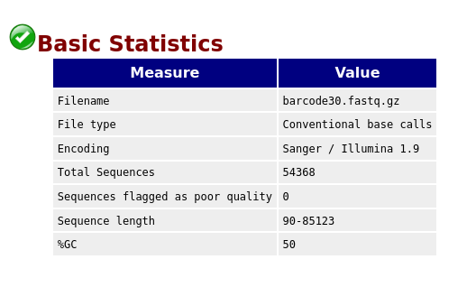
Basic Statistics
The first information you encounter is the basic statistics. The Basic Statistics module generates some simple composition statistics for the file analysed.
- Filename: The original filename of the file which was analysed
- File type: Says whether the file appeared to contain actual base calls or colorspace data which had to be converted to base calls
- Encoding: Says which ASCII encoding of quality values was found in this file.
- Total Sequences: A count of the total number of sequences processed. There are two values reported, actual and estimated. At the moment these will always be the same.
- Filtered Sequences: If running in Casava mode sequences flagged to be filtered will be removed from all analyses. The number of such sequences removed will be reported here. The total sequences count above will not include these filtered sequences and will the number of sequences actually used for the rest of the analysis.
- Sequence Length: Provides the length of the shortest and longest sequence in the set. If all sequences are the same length only one value is reported.
- %GC: The overall %GC of all bases in all sequences
Per Base Sequence Quality
The plot shows an overview of the range of quality values across all bases at each position in the FastQ file.
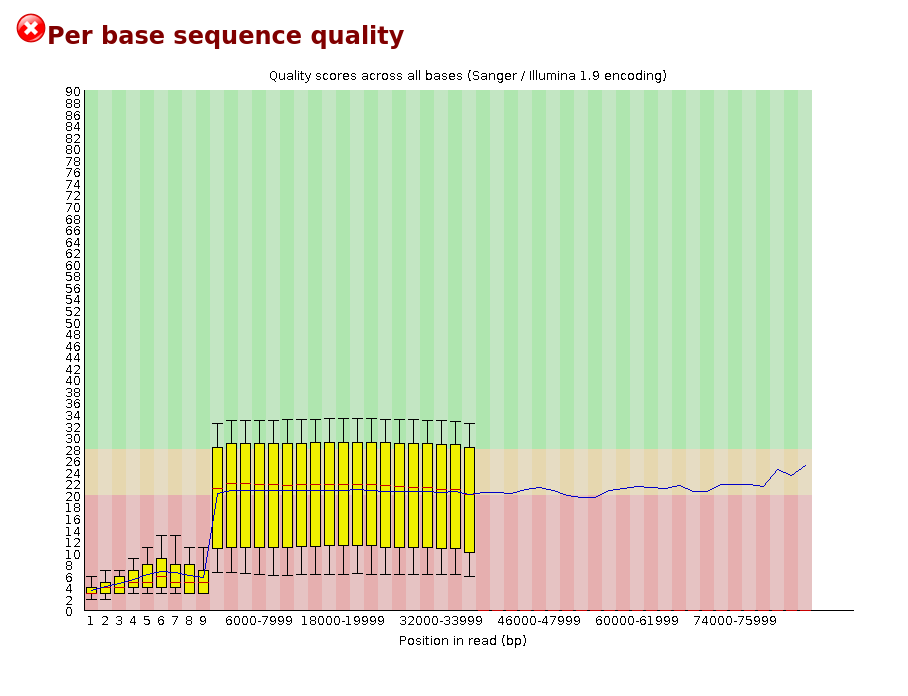
For each position a BoxWhisker type plot is drawn. The elements of the plot are as follows: - The central red line is the median value - The yellow box represents the inter-quartile range (25-75%) - The upper and lower whiskers represent the 10% and 90% points - The blue line represents the mean quality
The y-axis on the graph shows the quality scores. The higher the score the better the base call. The background of the graph divides the y-axis into very good quality calls (green), calls of reasonable quality (orange), and calls of poor quality (red). The quality of calls on most platforms will degrade as the run progresses, so it is common to see base calls falling into the orange area towards the end of a read.
It should be mentioned that there are number of different ways to encode a quality score in a FastQ file. FastQC attempts to automatically determine which encoding method was used, but in some very limited datasets it is possible that it will guess this incorrectly (ironically only when your data is universally very good!). The title of the graph will describe the encoding FastQC thinks your file used.
NB. Results from this module will not be displayed if your input is a BAM/SAM file in which quality scores have not been recorded.
Warning A warning will be issued if the lower quartile for any base is less than 10, or if the median for any base is less than 25.
Failure This module will raise a failure if the lower quartile for any base is less than 5 or if the median for any base is less than 20.
Common reasons for warnings
The most common reason for warnings and failures in this module is a general degradation of quality over the duration of long runs. In general sequencing chemistry degrades with increasing read length and for long runs you may find that the general quality of the run falls to a level where a warning or error is triggered.
If the quality of the library falls to a low level then the most common remedy is to perform quality trimming where reads are truncated based on their average quality. For most libraries where this type of degradation has occurred you will often be simultaneously running into the issue of adapter read-through so a combined adapter and quality trimming step is often employed.
Another possibility is that a warn / error is triggered because of a short loss of quality earlier in the run, which then recovers to produce later good quality sequence. This can happen if there is a transient problem with the run (bubbles passing through a flow cell for example). You can normally see this type of error by looking at the per-tile quality plot (if available for your platform). In these cases trimming is not advisable as it will remove later good sequence, but you might want to consider masking bases during subsequent mapping or assembly.
If your library has reads of varying length then you can find a warning or error is triggered from this module because of very low coverage for a given base range. Before committing to any action, check how many sequences were responsible for triggering an error by looking at the sequence length distribution module results.
Per Sequence Quality Scores
The per sequence quality score report allows you to see if a subset of your sequences have universally low quality values. It is often the case that a subset of sequences will have universally poor quality, often because they are poorly imaged (on the edge of the field of view etc), however these should represent only a small percentage of the total sequences.
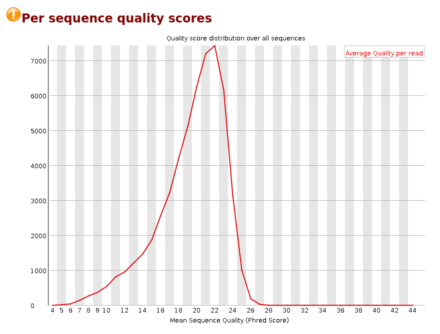
If a significant proportion of the sequences in a run have overall low quality then this could indicate some kind of systematic problem - possibly with just part of the run (for example one end of a flow cell).
NB. Results from this module will not be displayed if your input is a BAM/SAM file in which quality scores have not been recorded.
Warning A warning is raised if the most frequently observed mean quality is below 27 - this equates to a 0.2% error rate.
Failure An error is raised if the most frequently observed mean quality is below 20 - this equates to a 1% error rate.
Common reasons for warnings
This module is generally fairly robust and errors here usually indicate a general loss of quality within a run. For long runs this may be alleviated through quality trimming. If a bi-modal, or complex distribution is seen then the results should be evaluated in concert with the per-tile qualities (if available) since this might indicate the reason for the loss in quality of a subset of sequences.Per Base Sequence Content
Per Base Sequence Content plots out the proportion of each base position in a file for which each of the four normal DNA bases has been called.
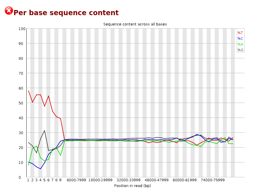
In a random library you would expect that there would be little to no difference between the different bases of a sequence run, so the lines in this plot should run parallel with each other. The relative amount of each base should reflect the overall amount of these bases in your genome, but in any case they should not be hugely imbalanced from each other.
It’s worth noting that some types of library will always produce biased sequence composition, normally at the start of the read. Libraries produced by priming using random hexamers (including nearly all RNA-Seq libraries) and those which were fragmented using transposases inherit an intrinsic bias in the positions at which reads start. This bias does not concern an absolute sequence, but instead provides enrichment of a number of different K-mers at the 5’ end of the reads. Whilst this is a true technical bias, it isn’t something which can be corrected by trimming and in most cases doesn’t seem to adversely affect the downstream analysis. It will however produce a warning or error in this module.
Warning This module issues a warning if the difference between A and T, or G and C is greater than 10% in any position.
Failure This module will fail if the difference between A and T, or G and C is greater than 20% in any position.
Common reasons for warnings
There are a number of common scenarios which would elicit a warning or error from this module.
Overrepresented sequences: If there is any evidence of overrepresented sequences such as adapter dimers or rRNA in a sample then these sequences may bias the overall composition and their sequence will emerge from this plot. Biased fragmentation: Any library which is generated based on the ligation of random hexamers or through tagmentation should theoretically have good diversity through the sequence, but experience has shown that these libraries always have a selection bias in around the first 12bp of each run. This is due to a biased selection of random primers, but doesn’t represent any individually biased sequences. Nearly all RNA-Seq libraries will fail this module because of this bias, but this is not a problem which can be fixed by processing, and it doesn’t seem to adversely affect the ability to measure expression. Biased composition libraries: Some libraries are inherently biased in their sequence composition. The most obvious example would be a library which has been treated with sodium bisulphite which will then have converted most of the cytosines to thymines, meaning that the base composition will be almost devoid of cytosines and will thus trigger an error, despite this being entirely normal for that type of library If you are analysing a library which has been aggressively adapter trimmed then you will naturally introduce a composition bias at the end of the reads as sequences which happen to match short stretches of adapter are removed, leaving only sequences which do not match. Sudden deviations in composition at the end of libraries which have undergone aggressive trimming are therefore likely to be spurious.[Per Sequence GC content]
We will talk more about GC content under identifying contaminiation. For now, let’s just have a look at our plot.
Per Base N Content
If a sequencer is unable to make a base call with sufficient confidence then it will normally substitute an N rather than a conventional base] call
This module plots out the percentage of base calls at each position for which an N was called.
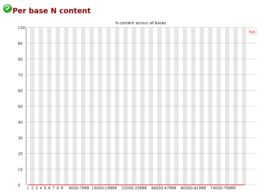
It’s not unusual to see a very low proportion of Ns appearing in a sequence, especially nearer the end of a sequence. However, if this proportion rises above a few percent it suggests that the analysis pipeline was unable to interpret the data well enough to make valid base calls.
Warning This module raises a warning if any position shows an N content of >5%.
Failure This module will raise an error if any position shows an N content of >20%.
Common reasons for warnings
The most common reason for the inclusion of significant proportions of Ns is a general loss of quality, so the results of this module should be evaluated in concert with those of the various quality modules. You should check the coverage of a specific bin, since it’s possible that the last bin in this analysis could contain very few sequences, and an error could be prematurely triggered in this case.
Another common scenario is the incidence of a high proportions of N at a small number of positions early in the library, against a background of generally good quality. Such deviations can occur when you have very biased sequence composition in the library to the point that base callers can become confused and make poor calls. This type of problem will be apparent when looking at the per-base sequence content results.I am sure by now, you will be bored with the many quality control tools. Now, let’s try our hands on some trimming to improve the quality of our sequences. To do this, we will use fastpand PoreChop.
fastp
click here to view the publication on fastp fastp is a tool designed to provide fast all-in-one pre-processing for FastQ files.
It is mostly used on short-reads illumina data ban can be applied to long-read ONT.
Features
- comprehensive quality profiling for both before and after filtering data (quality - curves, base contents, KMER, Q20/Q30, GC Ratio, duplication, adapter contents…)
- filter out bad reads (too low quality, too short, or too many N…)
- cut low quality bases for per read in its 5’ and 3’ by evaluating the mean quality - from a sliding window (like Trimmomatic but faster).
- trim all reads in front and tail
- cut adapters. Adapter sequences can be automatically detected, which means you don’t have to input the adapter sequences to trim them.
- correct mismatched base pairs in overlapped regions of paired end reads, if one base is with high quality while the other is with ultra low quality
- trim polyG in 3’ ends, which is commonly seen in NovaSeq/NextSeq data. Trim polyX in 3’ ends to remove unwanted polyX tailing (i.e. polyA tailing for mRNA-Seq data)
- preprocess unique molecular identifier (UMI) enabled data, shift UMI to sequence name.
- report JSON format result for further interpreting.
- visualize quality control and filtering results on a single HTML page (like FASTQC - but faster and more informative).
- split the output to multiple files (0001.R1.gz, 0002.R1.gz…) to support parallel - processing. Two modes can be used, limiting the total split file number, or limiting the lines of each split file.
- support long reads (data from PacBio / Nanopore devices).
- support reading from STDIN and writing to STDOUT
- support interleaved input
- support ultra-fast FASTQ-level deduplication
You can now go ahead and perform the fastp with the below command. We will perform the run on one of our Nanopore reads.
fastp --cut_front --cut_tail --trim_poly_x --cut_mean_quality 10 --qualified_quality_phred 10 --unqualified_percent_limit 10 --length_required 50 --in1 barcode30.fastq.gz --out1 barcode30.trim.fastq.gz --json barcode30_fastp.json --html barcode30_fastp.html --thread 4Detecting adapter sequence for read1...
No adapter detected for read1
Read1 before filtering:
total reads: 54368
total bases: 257262215
Q20 bases: 140726297(54.7015%)
Q30 bases: 59979993(23.3147%)
Read1 after filtering:
total reads: 2788
total bases: 13508368
Q20 bases: 9981247(73.8894%)
Q30 bases: 4923721(36.4494%)
Filtering result:
reads passed filter: 2788
reads failed due to low quality: 51575
reads failed due to too many N: 0
reads failed due to too short: 5
reads with adapter trimmed: 0
bases trimmed due to adapters: 0
reads with polyX in 3' end: 142
bases trimmed in polyX tail: 4340
Duplication rate (may be overestimated since this is SE data): 0%
JSON report: barcode30_fastp.json
HTML report: barcode30_fastp.html
fastp --cut_front --cut_tail --trim_poly_x --cut_mean_quality 10 --qualified_quality_phred 10 --unqualified_percent_limit 10 --length_required 50 --in1 barcode30.fastq.gz --out1 barcode30.trim.fastq.gz --json barcode30_fastp.json --html barcode30_fastp.html --thread 4
fastp v0.23.2, time used: 5 seconds
...You can also read out what is printed out on the terminal as a log file by passing the output to a textfile named fastp.log. This way, you don’t see all the long print out on the terminal.
fastp --cut_front --cut_tail --trim_poly_x --cut_mean_quality 10 --qualified_quality_phred 10 --unqualified_percent_limit 10 --length_required 50 --in1 barcode30.fastq.gz --out1 barcode30.trim.fastq.gz --json barcode30_fastp.json --html barcode30_fastp.html --thread 4 > fastp.logNote that the analysis perfomed above is just for demonstration purposes hence parameters set may not represent the true states.
You should now see three new files generated in your current directory.
barcode30.trim.fastq.gz
barcode30_fastp.json
barcode30_fastp.html
Now let’s go ahead and see what our output looks like by opening the barcode30_fastp.html file. You should be able to interpret the output by now.
Note that the date presented below are just for demonstration purposes adn do not represent the actual data from the barcode30.fastq.gz reads.
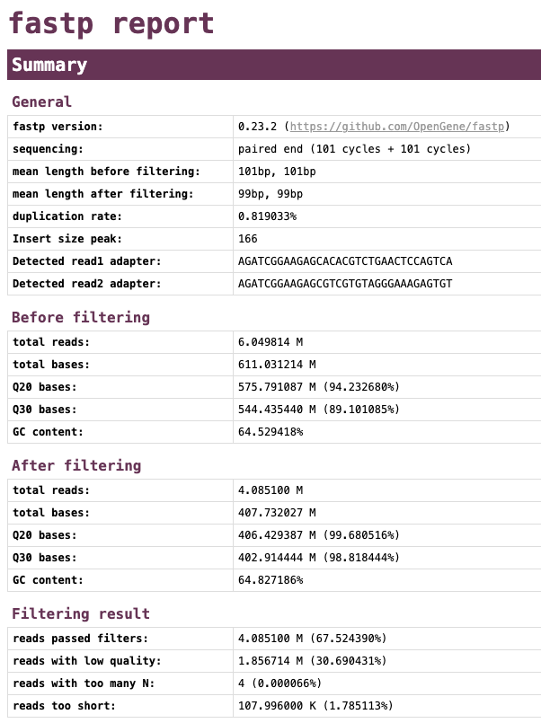
Let’s have a look at the quality of the reads before and after trimming. What obvious differences do you notice?
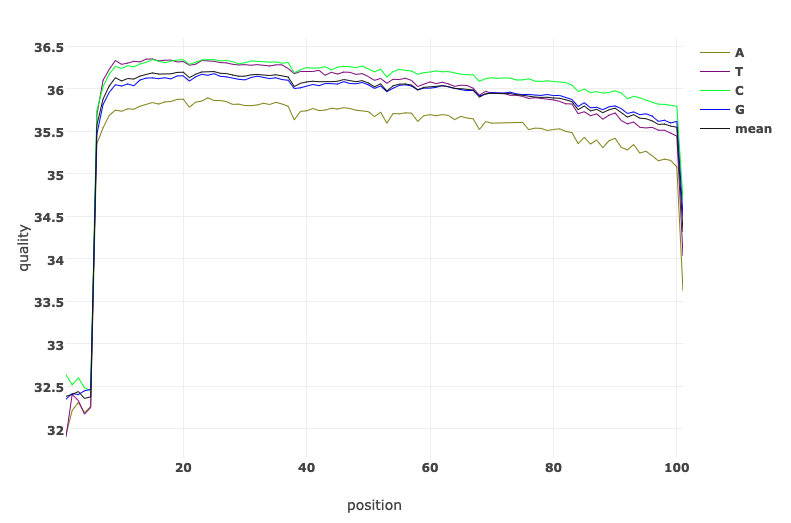
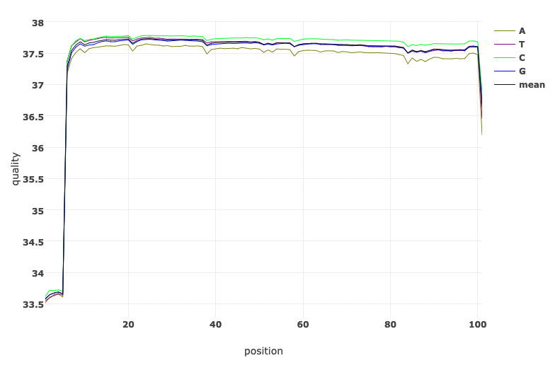
Read Quality before and after fastp processing
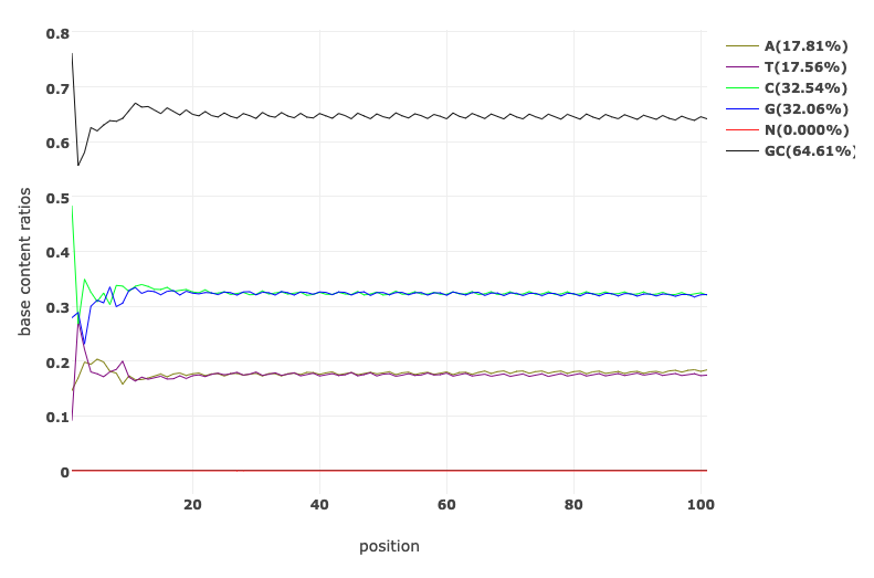
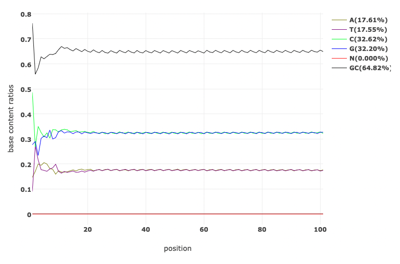
Base Content Quality before and after fastp processing
PoreChop
![]()
Porechop is a tool for finding and removing adapters from Oxford Nanopore reads. Adapters on the ends of reads are trimmed off, and when a read has an adapter in its middle, it is treated as chimeric and chopped into separate reads. Porechop performs thorough alignments to effectively find adapters, even at low sequence identity.
How it works
Find matching adapter sets
Porechop first aligns a subset of reads (default 10000 reads, change with --check_reads) to all known adapter sets. Adapter sets with at least one high identity match (default 90%, change with --adapter_threshold) are deemed present in the sample.
Identity in this step is measured over the full length of the adapter. E.g. in order to qualify for a 90% match, an adapter could be present at 90% identity over its full length, or it could be present at 100% identity over 90% of its length, but a 90% identity match over 90% of the adapter length would not be sufficient.
The alignment scoring scheme used in this and subsequent alignments can be modified using the --scoring_scheme option (default: match = 3, mismatch = -6, gap open = -5, gap extend = -2).
Trim adapters from read ends
The first and last bases in each read (default 150 bases, change with --end_size) are aligned to each present adapter set. When a long enough (default 4, change with --min_trim_size) and strong enough (default 75%, change with –end_threshold) match is found, the read is trimmed. A few extra bases (default 2, change with --extra_end_trim) past the adapter match are removed as well to ensure it’s all removed.
Identity in this step is measured over the aligned part of the adapter, not its full length. E.g. if the last 5 bases of an adapter exactly match the first 5 bases of a read, that counts as a 100% identity match and those bases will be trimmed off. This allows Porechop to effectively trim partially present barcodes.
The default --end_threshold is low (75%) because false positives (trimming off some sequence that wasn’t really an adapter) shouldn’t be too much of a problem with long reads, as only a tiny fraction of the read is lost.
Split reads with internal adapters
The entirety of each read is aligned to the present adapter sets to spot cases where an adapter is in the middle of the read, indicating a chimera. When a strong enough match is found (default 85%, change with --middle_threshold), the read is split. If the resulting parts are too short (default less than 1000 bp, change with --min_split_read_size), they are discarded.
The default --middle_threshold (85%) is higher than the default --end_threshold (75%) because false positives in this step (splitting a read that is not chimeric) could be more problematic than false positives in the end trimming step. If false negatives (failing to split a chimera) are worse for you than false positives (splitting a non-chimera), you should reduce this threshold (e.g. --middle_threshold 75).
Extra bases are also removed next to the hit, and how many depends on the side of the adapter. If we find an adapter that’s expected at the start of a read, it’s likely that what follows is good sequence but what precedes it may not be. Therefore, a few bases are trimmed after the adapter (default 10, change with --extra_middle_trim_good_side) and more bases are trimmed before the adapter (default 100, change with --extra_middle_trim_bad_side). If the found adapter is one we’d expect at the end of the read, then the “good side” is before the adapter and the “bad side” is after the adapter.
Here is a real example of the “good” and “bad” sides of an adapter. The adapter is in the middle of this snippet (SQK-NSK007_Y_Top at about 90% identity). The bases to the left are the “bad” side and their repetitive nature is clear. The bases to the right are the “good” side and represent real biological sequence.
TGTTGTTGTTGTTATTGTTGTTATTGTTGTTGTATTGTTGTTATTGTTGTTGTTGTACATTGTTATTGTTGTATTGTTGTTATTGTTGTTGTATTATCGGTGTACTTCGTTCAGTTACGTATTACTATCGCTATTGTTTGCAGTGAGAGGTGGCGGTGAGCGTTTTCAAATGGCCCTGTACAATCATGGGATAACAACATAAGGAACGGACCATGAAGTCACTTCTDiscard reads with internal adapters
If you run Porechop with --discard_middle, the reads with internal adapters will be thrown out instead of split.
If you plan on using your reads with Nanopolish, then the --discard_middle option is required. This is because Nanopolish first runs nanopolish index to find a one-to-one association between FASTQ reads and fast5 files. If you ran Porechop without --discard_middle, then you could end up with multiple separate FASTQ reads which are from a single fast5, and this is incompatible with Nanopolish.
This option is also recommended if you are trimming reads from a demultiplexed barcoded sequencing run. This is because chimeric reads may contain two sequences from two separate barcodes, so throwing them out is the safer option to reduce cross-barcode contamination.
Porechop can perform a lot of other very important analysis including demultiplexing. You can find more by following this link.
For now let’s make our hands dry by performing porechop on any of our reads.
We see from our run, three basic analysis:
- Trimming adapter from the reads
- Splitting reads containing adapter
- saving trimed reads to file
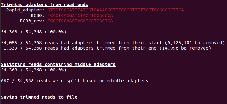
Also take time to go throught the list of adapters. Do you see anything unusual?
Hint
You will find that only the adapters used for your samples are highlightedKnown issues
Adapter search
Porechop tries to automatically determine which adapters are present by looking at the reads, but this approach has a few issues:
- As the number of kits/barcodes has grown, adapter-search as part of the Porechop’s pipeline has become increasingly slow.
- Porechop only does the adapter search on a subset of reads, which means there can be problems with non-randomly ordered read sets (e.g. all barcode 1 reads at the start of a file, followed by barcode 2 reads, etc).
- Many ONT adapters share common sequence with each other, making false positive adapter finds possible.
2.1.5 Identifying contamination
It is always a good idea to check that your data is from the species you expect it to be. A very useful tool for this is Kraken. In this workshop we will go through how you can use Kraken to check your samples for contamination.
Kraken 2
click here to view the publication on Kraken 2 kraken is a taxonomic sequence classifier that assigns taxonomic labels to DNA sequences. Kraken examines the k-mers within a query sequence and uses the information within those k-mers to query a database. That database maps k-mers to the lowest common ancestor (LCA) of all genomes known to contain a given k-mer.
The first version of Kraken used a large indexed and sorted list of -mer/LCA pairs as its database. While fast, the large memory requirements posed some problems for users, and so Kraken 2 was created to provide a solution to those problems.
To run Kraken 2, you need to provide the path to the database. By default, the input files are assumed to be in FASTA format, so in this case we also need to tell Kraken that our input files are in FASTQ format, gzipped, and that they are ONT reads.
You can now go ahead and run Kraken 2 with the below command.
Take note of these: 1. You have to specify the directory to the database 2. Our input files will be the porechopped fastq sequences from the fastp analysis.
Do this to run Kraken 2:
kraken2 --db ../database/minikraken2_v1_8GB --threads 8 --unclassified-out barcode30.unclassified#.fastq --classified-out barcode30.classified#.fastq --report barcode30.kraken2.report.txt --output barcode30.kraken2.out --gzip-compressed --report-zero-counts barcode30_porechopped.fastq.gzLoading database information... done.
53949 sequences (251.01 Mbp) processed in 30.316s (106.8 Kseq/m, 496.79 Mbp/m).
51565 sequences classified (95.58%)
2384 sequences unclassified (4.42%)You should now see some new files generated in your current directory. How many new files have been generated? Do you see that the fastq files are unzipped?
You can try to read the two kraken report output text files created, but I’m sure that won’t make real sense to you.
Quick look at Kraken 2 report
Run the command to have a quick look at the Kraken 2 report.
head -n 20 barcode30.kraken2.report.txtThe six columns in this file are:
- Percentage of reads covered by the clade rooted at this taxon
- Number of reads covered by the clade rooted at this taxon
- Number of reads assigned directly to this taxon
- A rank code, indicating (U)nclassified, (D)omain, (K)ingdom, (P)hylum, (C)lass, (O)rder, (F)amily, (G)enus, or (S)pecies. All other ranks are simply ‘-’.
- NCBI taxonomy ID
- Scientific name
Just like we did for the fastq-scan output, we will have to convert the Kraken 2 output to a more readable format. Before we do this, we will have to perform one more analysis on our sample. The Kraken 2 often does not provide exhaustive results. To re-estimate taxonomic abundance of the samples we have to do this with another tool called Bracken using the output of Kraken 2.
Bracken
click here to view the publication on Bracken Bracken is a companion program to Kraken 1, KrakenUniq, or Kraken 2 While Kraken classifies reads to multiple levels in the taxonomic tree, Bracken allows estimation of abundance at a single level using those classifications (e.g. Bracken can estimate abundance of species within a sample)
You can now go ahead and perform Bracken with the below command.
Run Bracken with the following command:
bracken -l S -t 10 -d ../database/minikraken2_v1_8GB -i barcode30.kraken2.report.txt -o barcode30_bracken_S.tsv>> Checking for Valid Options...
>> Running Bracken
>> python src/est_abundance.py -i barcode30.kraken2.report.txt -o barcode30_bracken_S.tsv -k ../database/minikraken2_v1_8GB/database100mers.kmer_distrib -l S -t 10
PROGRAM START TIME: 08-09-2023 17:20:28
>> Checking report file: barcode30.kraken2.report.txt
BRACKEN SUMMARY (Kraken report: barcode30.kraken2.report.txt)
>>> Threshold: 10
>>> Number of species in sample: 11780
>> Number of species with reads > threshold: 10
>> Number of species with reads < threshold: 11770
>>> Total reads in sample: 53949
>> Total reads kept at species level (reads > threshold): 16065
>> Total reads discarded (species reads < threshold): 273
>> Reads distributed: 35185
>> Reads not distributed (eg. no species above threshold): 42
>> Unclassified reads: 2384
BRACKEN OUTPUT PRODUCED: barcode30_bracken_S.tsv
PROGRAM END TIME: 08-09-2023 17:20:28
Bracken complete.
You should now see two new files generated in your current directory. You can take a look at them as they are small files. You can already guess what specie we are working with from the barcode30_bracken_S.tsv file.
Producing a more friendly species composition file
Imagine you have over 100 samples and have produced Bracken output files for each file using a simple bash script. Ho do you check each individual file to see what species abundance there is? This will be tedious right? How can we make things easier for us? For instance have them all in one .tsv file to examine at a go. Your guess is as good as mine. …Let’s write a script for that.
To do this, we can simply parse all the Kraken 2 and Bracken results into a more friendly .tsv file that summarises all the output into one file. We will achieve this with a simple python script.
Parse Kraken 2 and Bracken results files into tsv format
We will run a simple python script to achieve this purpose. In your working directory, you will find a file named kraken_parser.py. This is a simple python script that will do the job for us.
We can go ahead and execute that python script by running the command below:
python kraken_parser.pyYou should now see another file generated in your directory called Bracken_species_composition.tsv.
Now let’s go ahead and have a look at the tsv file with the command below. Remember, we have run analysis on only one sample and so will expect only one line of results.
Alternatively, you can open the tsv file with any appropriate GUI software (excel or libreoffice)
Now, what if we want to also see all the QC statistics in one go provided we performed the analysis for multiple samples (or in our case even for just one sample).
Thankfully, bioinformaticians are not sleeping, there is one final tool (MultiQC) we will discuss here which puts all that analysis we have performed into a single report that is viewable on a web browser, yes an .html file.
MultiQC
click here to view the publication on MultiQC or check out their website
MultiQC is a tool to create a single report with interactive plots for multiple bioinformatics analyses across many samples.
Reports are generated by scanning given directories for recognised log files. These are parsed and a single HTML report is generated summarising the statistics for all logs found. MultiQC reports can describe multiple analysis steps and large numbers of samples within a single plot, and multiple analysis tools making it ideal for routine fast quality control.
Do this to get the help information for multiqc
multiqc -h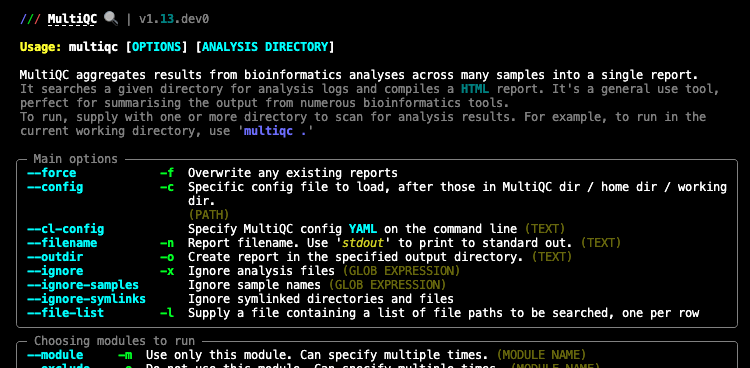
You can now go ahead and perform the MultiQC with the below command. We will only add the -f flag which overwrites any existing MultiQC reports.
Perform the analysis with this command:
multiqc -f .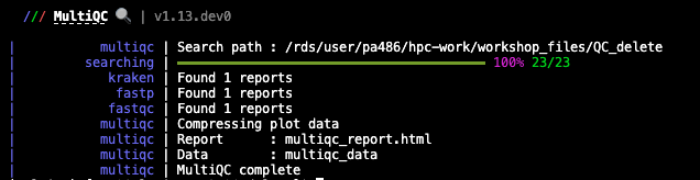
The report is created in multiqc_report.html by default. Tab-delimited data files are also created in a directory called multiqc_data/, containing extra information. These can be easily inspected using Excel.
You should now see two new files generated in your current directory.
Let’s have a quick look the report by simply opening it in a web browser.
We should now know what each plot represent. If you don’t at this point, then you may want to start from the beginning of this document.
2.1.6 QC bash script: Putting it all together
Now let’s try this out! We will generate QC stats for all five Nanopore reads. We will perform all the analysis above (except fastp) in one run while generating all the various files at each stage within the pipeline in tandem.
Running multiple samples with a simple bash script
All the fastq files needed for this analysis are located in the current working QC directory. You can have a look by simply running the below command to check out all the reads present in the current directory.
Let’s have a look at the QC bash script we are going to run:
cat qcloop_ont.shThe script contains several commands, some are combined together using pipes. (UNIX pipes is a very powerful and elegant concept which allows us to feed the output of one command into the next command and avoid writing intermediate files. If you are not comfortable with UNIX or how scripts look like and how they work, consider having a go at the UNIX tutorial or more specifically bonus shell script.
Now run the script to create the QC stats (this may take a while):
The script will produce all the intermediate and final files we have encountered in this session.
Perform a simple ls command with the arguments -lhrt and view the most recent files created.
ls -lhrtWhich files do you consider most useful?
Now, let’s have a look at the two most important files here — The multiqc_report.html and the Bracken_species_composition.tsv.
If you have successfully gone through the exercise above, congratulations!!! You are a bioinformatics QC expert now.
Now, let’s take particular note of the porechopped genomes that we are most confident in. We will carry out our de novo assembly of long reads from these genomes in our next lesson.
Disk Usage II — Cleaning up after analysis
Now that we are done investigating our genomic sequences, let’s pause again and check the space of our current working directory.
You can do this with the disk usage du command
du -hHow much disk space have you used since the start of the analysis? I’m sure it’s more than 4G. That’s fine. Let’s do some cleaning up. We will remove rm all files that we may not need for further analysis. Most of these files are intermediate files and can always be reproduced if we need to.
You will find this cleaning process very useful in the next chapter where we will generate tonnes and tonnes of data.
remove all porechopped fastq files if not needed
rm *porechopped*remove all classified and unclassified fastq files if not needed
rm *classified*remove all Kraken 2 output if not needed
rm *kraken2.out2.1.7 deactivate qc_ont environment
Now that we are done with all our analysis, let’s deactivate the qc_ont environment:
mamba deactivate2.1.8 Credit
Information on this page has been adapted and modified from the following source(s):
https://github.com/sanger-pathogens/QC-training
https://github.com/wdecoster/NanoPlot
https://github.com/rpetit3/fastq-scan
https://www.bioinformatics.babraham.ac.uk/projects/fastqc/
https://github.com/OpenGene/fastp
https://github.com/rrwick/Porechop
https://github.com/DerrickWood/kraken2
https://github.com/jenniferlu717/Bracken
https://github.com/ewels/MultiQC