2.2 Assembly

Teaching: 90 min || Exercises: 30 min
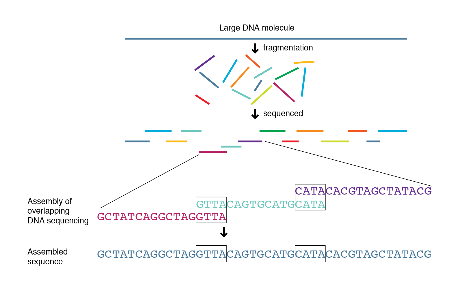
Overview

Questions:
  • What is de novo genome assembly?
  • What is reference-based assembly?
  • How do I assemble my genome using ONT data?
  • How do I assess the quality of my assembled genome?
Learning Objectives:
  • Understand what de novo genome assembly is and how it differs from reference-based assembly.
  • Assemble sequence data with flye and polish with medaka
  • Generate metrics for your assembly with QUAST
Key Points:
  • Best practice assembly and polishing tools for Nanopore data include
  • de novo genome assembly involves assembling a genome from the raw reads without the aid of a reference genome as against a reference-based assembly which relies on a reference genome for alignment and subsequent assembly

2.2.1 Background

There are two approaches for genome assembly: reference-based (or comparative) or de novo. In a reference-based assembly, we use a reference genome as a guide to map our sequence data to and thus reassemble our sequence this way (we will not do this here with our ONT data but will try it out with illumina data later on in the course). Alternatively, we can create a ‘new’ (de novo) assembly that does not rely on a map or reference and more closely reflects the actual genome structure of the isolate that was sequenced.

Genome assembly

Genome assemblers

Several tools are available for de novo genome assembly depending on whether you’re trying to assemble short-read sequence data, long reads or else a combination of both. Three of the most commonly used assemblers for long read data are Flye, Unicycler and Miniasm.

Now that we have been able to see how Quality our Nanopore sequences are, we can can confidently proceed to assemble our bacterial genome. Here, we will perform long read assembly utilizing Flye in combination with Medaka. Other useful tools for assembly includes Unicycler and Miniasm in combination with Racon, or Canu. Another polishing tool in addition to Medaka is NanoPolish with Fast5 files. Each of these tools, have their pros and cons but we will not go deep into them here. Following the assembly, we will QC the products using QUAST.

Disk Usage I — Before analysis

Before we start performing any assemblies, let’s pause and check the space of our current working directory as we did for our previous lesson.

You can do this with the disk usage du command

du -h
Current Disk Space In assembly_annotation_MTB Directory ~247MB
Now, keep this value in mind, and this time, don’t forget it. We will come back to it at the end of this chapter.

2.2.3 Assembly and Genome Polishing

de novo genome assembly with Flye

Flye is a de novo assembler for single-molecule sequencing reads, such as those produced by PacBio and Oxford Nanopore Technologies. It is designed for a wide range of datasets, from small bacterial projects to large mammalian-scale assemblies. The package represents a complete pipeline: it takes raw PacBio / ONT reads as input and outputs polished contigs. Flye also has a special mode for metagenome assembly.

Nanopore assemblers are still in development, but Flye is a de facto standard.

Help

Do this to get the help information for flye

flye -h
usage: flye (--pacbio-raw | --pacbio-corr | --pacbio-hifi | --nano-raw |
         --nano-corr | --nano-hq ) file1 [file_2 ...]
         --out-dir PATH

         [--genome-size SIZE] [--threads int] [--iterations int]
         [--meta] [--polish-target] [--min-overlap SIZE]
         [--keep-haplotypes] [--debug] [--version] [--help]
         [--scaffold] [--resume] [--resume-from] [--stop-after]
         [--read-error float] [--extra-params]
         [--deterministic]

Assembly of long reads with repeat graphs

options:
  -h, --help            show this help message and exit
  --pacbio-raw path [path ...]
                        PacBio regular CLR reads (<20% error)

...

Usage

The general format of the command is:

flye  --nano-raw file1 [file_2 ...] --out-dir PATH

We will attempt to start flye by running the below command on our first dataset barcode30. Note that, here we will use our trimmed dataset barcode30_porechopped.fastq.gz.

flye  --nano-raw barcode30_porechopped.fastq.gz --out-dir barcode30_flye
[2023-08-10 09:28:51] INFO: Starting Flye 2.9.2-b1786
[2023-08-10 09:28:51] INFO: >>>STAGE: configure
[2023-08-10 09:28:51] INFO: Configuring run
[2023-08-10 09:28:55] INFO: Total read length: 251007904
[2023-08-10 09:28:55] INFO: Reads N50/N90: 8665 / 2409
[2023-08-10 09:28:55] INFO: Minimum overlap set to 2000
[2023-08-10 09:28:55] INFO: >>>STAGE: assembly
[2023-08-10 09:28:55] INFO: Assembling disjointigs
[2023-08-10 09:28:56] INFO: Reading sequences
[2023-08-10 09:29:03] INFO: Counting k-mers:
0% 10% 20% 30% 40% 50% 60% 70% 80% 90% 100%
[2023-08-10 09:30:52] INFO: Filling index table (1/2)
0% 10% 20% 30% 40% 50% 60% 70% 80% 90% 100%
[2023-08-10 09:32:37] INFO: Filling index table (2/2)
0% 10% 20% 30% 40% 50% 60% 70% 80% 90% 100%
[2023-08-10 09:35:43] INFO: Extending reads
[2023-08-10 09:37:04] INFO: Overlap-based coverage: 38
[2023-08-10 09:37:04] INFO: Median overlap divergence: 0.073935
...
...
[2023-08-10 09:53:46] INFO: Alignment error rate: 0.074446
[2023-08-10 09:53:46] INFO: Correcting bubbles
0% 10% 20% 30% 40% 50% 60% 70% 80% 90% 100%
[2023-08-10 09:59:12] INFO: >>>STAGE: finalize
[2023-08-10 09:59:12] INFO: Assembly statistics:

    Total length:   5551201
    Fragments:  14
    Fragments N50:  3514571
    Largest frg:    3514571
    Scaffolds:  0
    Mean coverage:  44

NB. If the input reads were corrected, use --nano-corr instead of --nano-raw.

The following files will be created in the barcode30_flye directory:

Relevant output files Description
assembly.fasta The final assembly you should use
assembly_info.txt Contig summary information
assembly_graph.gfa Assembly graph
flye.log Full log file for bug reporting

Let’s have quick look at the assembly_info.txt file and attempt to explain it’s contents.

Peep into assembly_info.txt
cat barcode30_flye/assembly_info.txt
#seq_name   length  cov.    circ.   repeat  mult.   alt_group   graph_path
contig_2    3514571 41  N   N   1   *   -3,2,-3
contig_1    1663577 45  N   N   1   *   3,1,3
contig_10   141945  29  Y   N   1   *   10
contig_16   81727   39  Y   N   1   *   16
contig_5    46307   54  N   Y   1   6   *,5,*
contig_3    42686   42  N   Y   1   *   3
contig_4    17614   12  N   Y   1   6   *,4,*
contig_18   9539    797 Y   Y   19  *   18
contig_14   8359    18  N   Y   3   8   *,14,*
contig_9    8110    1108    N   Y   26  *   9
contig_12   5813    22  N   Y   1   *   12
contig_17   5810    41  N   Y   1   *   17
contig_6    4632    10  N   N   10  *   *,6,*
contig_8    511 49  Y   Y   1   2   8

We can obtain most of the above information by just applying very simple commandline tools to interogate the assembly.fasta file.

Exercise 2.2.1: Obtain statistics from assembly.fasta file.
  1. What simple command can you use to have a peep into the assembly.fasta file by looking at only the first 10 lines.

  2. What quick command can you use to count all the lines and letters in the assembly.fasta file.

  3. With one line of command, how would you determine the number of contigs present in the assembly.fasta file.

Report on your findings. How do they varry from the information contained in the assembly_info.txt file.

  1. To view the first 10 lines:
head -n 10 assembly.fasta

To view the last 10 lines

tail -n 10 assembly.fasta
wc assembly.fasta
grep -c '>' assembly.fasta

Before we move on to the next step, let’s rename our assembly (assembly.fasta) to something more meaningful barcode30_assembly.fasta and copy it to the current directory.

How do we do this?

cp barcode30_flye/assembly.fasta barcode30_assembly.fasta

genome polishing with Medaka

Now that we are done with flye, let’s deactivate the flye environment and activate our medaka environment.

mamba deactivate
mamba activate medaka

Medaka is an assembly polisher and variant caller made by ONT and used to create consensus sequences and variant calls from nanopore sequencing data. It is the recommended polisher for Flye assemblies. The Medaka documentation mentions that it has specifically been trained on Flye output (it is an ML-based tool).

Medaka requires only basecalled data — .fasta or .fastq and it is 50X faster than Nanopolish.

Help

Do this to get the help information for Medaka

medaka -h
usage: medaka [-h] [--version]
              {compress_bam,features,train,consensus,smolecule,consensus_from_features,fastrle,stitch,variant,snp,tools}
              ...

options:
  -h, --help            show this help message and exit
  --version             show program's version number and exit

subcommands:
  valid commands

  {compress_bam,features,train,consensus,smolecule,consensus_from_features,fastrle,stitch,variant,snp,tools}
                        additional help
    compress_bam        Compress an alignment into RLE form.
    features            Create features for inference.
    train               Train a model from features.
    consensus           Run inference from a trained model and alignments.
    smolecule           Create consensus sequences from single-molecule reads.
    consensus_from_features
                        Run inference from a trained model on existing features.
    fastrle             Create run-length encoded fastq (lengths in quality track).
    stitch              Stitch together output from medaka consensus into final output.
    variant             Decode probabilities to VCF.
    snp                 Decode probabilities to SNPs.
    tools               tools subcommand.

Usage

The general format of the command is:
medaka_consensus -i ${BASECALLS} -d ${DRAFT} -o ${OUTDIR} -t ${NPROC} -m r941_min_high_g303 

We will polish our flye assembly by running the following command:

Polish flye output
medaka_consensus -i barcode30_porechopped.fastq.gz -d barcode30_assembly.fasta -o barcode30_medaka -t 8 -m r10_min_high_g340
Checking program versions
This is medaka 1.8.0
Program    Version    Required   Pass     
bcftools   1.17       1.11       True     
bgzip      1.17       1.11       True     
minimap2   2.26       2.11       True     
samtools   1.17       1.11       True     
tabix      1.17       1.11       True     
Aligning basecalls to draft
...
...
[12:55:23 - PWorker] Processed 3 batches
[12:55:23 - PWorker] All done, 0 remainder regions.
[12:55:23 - Predict] Finished processing all regions.
[12:55:25 - DataIndx] Loaded 1/1 (100.00%) sample files.
[12:55:25 - DataIndx] Loaded 1/1 (100.00%) sample files.
[12:55:25 - DataIndx] Loaded 1/1 (100.00%) sample files.
[12:55:25 - DataIndx] Loaded 1/1 (100.00%) sample files.
[12:55:25 - DataIndx] Loaded 1/1 (100.00%) sample files.
[12:55:25 - DataIndx] Loaded 1/1 (100.00%) sample files.
[12:55:25 - DataIndx] Loaded 1/1 (100.00%) sample files.
[12:55:25 - DataIndx] Loaded 1/1 (100.00%) sample files.
[12:55:25 - DataIndx] Loaded 1/1 (100.00%) sample files.
[12:55:25 - TrimOlap] disjointig_2:22835.0-30849.0 and disjointig_2:85459.0-91200.0 cannot be concatenated as there is no overlap and they do not abut.
[12:55:25 - DataIndx] Loaded 1/1 (100.00%) sample files.
[12:55:25 - TrimOlap] disjointig_3:63937.0-73640.0 and disjointig_3:78942.0-88372.0 cannot be concatenated as there is no overlap and they do not abut.
[12:55:25 - TrimOlap] disjointig_1:4078692.0-4088250.0 and disjointig_1:4088272.0-4098065.0 cannot be concatenated as there is no overlap and they do not abut.
[12:55:25 - TrimOlap] disjointig_1:4124178.0-4133945.0 and disjointig_1:4133977.0-4143803.0 cannot be concatenated as there is no overlap and they do not abut.
Polished assembly written to barcode30_medaka/consensus.fasta, have a nice day.
Tip

If Medaka runs out of memory, add option -b 80 to the command-line. If it still runs out of memory, reduce the 80 further until it doesn’t.

Just like we did for the assembly.fasta file generated from flye, let’s rename the consensus.fasta file to a more meaningful name.

Rename consensus file and copy to current directory
cp barcode30_medaka/consensus.fasta barcode30_polished_assembly.fasta
Setting the righ model -m.

For best results it is important to specify the correct model, -m in the above command we just run, according to the basecaller used. Allowed values can be found by running medaka tools list\_models.

Medaka models are named to indicate

  • the pore type,
  • the sequencing device (MinION or PromethION),
  • the basecaller variant,
  • the basecaller version, with the format:
{pore}_{device}_{caller variant}_{caller version}

For example the model named r941_min_fast_g303 should be used with data from MinION (or GridION) R9.4.1 flowcells using the fast Guppy basecaller version 3.0.3. By contrast the model r941_prom_hac_g303 should be used with PromethION data and the high accuracy basecaller (termed “hac” in Guppy configuration files). Where a version of Guppy has been used without an exactly corresponding medaka model, the medaka model with the highest version equal to or less than the guppy version should be selected.

Bacterial (ploidy-1) variant calling

Note that we can perform variant calling with medaka. Variant calling for monoploid samples is enabled through the medaka_haploid_variant workflow:

medaka_haploid_variant -i <reads.fastq> -r <ref.fasta>

This requires the reads as a .fasta or .fastq and a reference sequence as a .fasta file.

2.2.4 Assembly quality assessment with QUAST

Now that we are done with medaka, let’s deactivate the medaka environment and activate our quast environment.

mamba deactivate
mamba activate quast

Genome assembly evaluation tool

Before we do any further analyses with our assemblies, we need to assess the quality. To do this we use a tool called QUAST. QUAST stands for QUality ASsessment Tool. It evaluates genome/metagenome assemblies by computing and generating various metrics for assemblies.

These include but aren’t limited to:

  1. The total number of contigs greater than 0 bp. Ideally, we like to see assemblies in the smallest number of contigs (‘pieces’) as this means there is likely less missing data contained in gaps between contigs.
  2. The total length of the assembly. We normally know what the expected length of our assembly is (for more diverse organisms like E. coli there may be a range of genome sizes). The length of your assembly should be close to the expected genome size. If it’s too big or too small, either there is some kind of contamination or else you’ve sequenced the wrong species!
  3. The N50 of the assembly. This is the final metric often used to assess the quality of an assembly. The N50 is typically calculated by averaging the length of the largest contigs that account for 50% of the genome size. This is a bit more complicated conceptually but the higher the N50 the better. A large N50 implies that you have a small number of larger contigs in your assembly which equals a good assembly.

We will run quast in the same assembly environment.

Help

Do this to get the help information for QUAST:

quast -h
QUAST: Quality Assessment Tool for Genome Assemblies
Version: 5.2.0

Usage: python /home/ajv37/.conda/envs/quast/bin/quast [options] <files_with_contigs>

Options:
-o  --output-dir  <dirname>       Directory to store all result files [default: quast_results/results_<datetime>]
-r                <filename>      Reference genome file
-g  --features [type:]<filename>  File with genomic feature coordinates in the reference (GFF, BED, NCBI or TXT)
                                  Optional 'type' can be specified for extracting only a specific feature type from GFF
-m  --min-contig  <int>           Lower threshold for contig length [default: 500]
-t  --threads     <int>           Maximum number of threads [default: 25% of CPUs]

Advanced options:
-s  --split-scaffolds                 Split assemblies by continuous fragments of N's and add such "contigs" to the comparison
-l  --labels "label, label, ..."      Names of assemblies to use in reports, comma-separated. If contain spaces, use quotes
-L                                    Take assembly names from their parent directory names
-e  --eukaryote                       Genome is eukaryotic (primarily affects gene prediction)
    --fungus                          Genome is fungal (primarily affects gene prediction)
    --large                           Use optimal parameters for evaluation of large genomes
                                      In particular, imposes '-e -m 3000 -i 500 -x 7000' (can be overridden manually)
-k  --k-mer-stats                     Compute k-mer-based quality metrics (recommended for large genomes)
                                      This may significantly increase memory and time consumption on large genomes
    --k-mer-size                      Size of k used in --k-mer-stats [default: 101]
    --circos                          Draw Circos plot
-f  --gene-finding                    Predict genes using GeneMarkS (prokaryotes, default) or GeneMark-ES (eukaryotes, use --eukaryote)
    --mgm                             Use MetaGeneMark for gene prediction (instead of the default finder, see above)
    --glimmer                         Use GlimmerHMM for gene prediction (instead of the default finder, see above)
    --gene-thresholds <int,int,...>   Comma-separated list of threshold lengths of genes to search with Gene Finding module
                                      [default: 0,300,1500,3000]
    --rna-finding                     Predict ribosomal RNA genes using Barrnap
-b  --conserved-genes-finding         Count conserved orthologs using BUSCO (only on Linux)
    --operons  <filename>             File with operon coordinates in the reference (GFF, BED, NCBI or TXT)
    --est-ref-size <int>              Estimated reference size (for computing NGx metrics without a reference)
    --contig-thresholds <int,int,...> Comma-separated list of contig length thresholds [default: 0,1000,5000,10000,25000,50000]
-u  --use-all-alignments              Compute genome fraction, # genes, # operons in QUAST v1.* style.
                                      By default, QUAST filters Minimap's alignments to keep only best ones
-i  --min-alignment <int>             The minimum alignment length [default: 65]
    --min-identity <float>            The minimum alignment identity (80.0, 100.0) [default: 95.0]
-a  --ambiguity-usage <none|one|all>  Use none, one, or all alignments of a contig when all of them
                                      are almost equally good (see --ambiguity-score) [default: one]
    --ambiguity-score <float>         Score S for defining equally good alignments of a single contig. All alignments are sorted 
                                      by decreasing LEN * IDY% value. All alignments with LEN * IDY% < S * best(LEN * IDY%) are 
                                      discarded. S should be between 0.8 and 1.0 [default: 0.99]
    --strict-NA                       Break contigs in any misassembly event when compute NAx and NGAx.
                                      By default, QUAST breaks contigs only by extensive misassemblies (not local ones)
-x  --extensive-mis-size  <int>       Lower threshold for extensive misassembly size. All relocations with inconsistency
                                      less than extensive-mis-size are counted as local misassemblies [default: 1000]
    --scaffold-gap-max-size  <int>    Max allowed scaffold gap length difference. All relocations with inconsistency
                                      less than scaffold-gap-size are counted as scaffold gap misassemblies [default: 10000]
    --unaligned-part-size  <int>      Lower threshold for detecting partially unaligned contigs. Such contig should have
                                      at least one unaligned fragment >= the threshold [default: 500]
    --skip-unaligned-mis-contigs      Do not distinguish contigs with >= 50% unaligned bases as a separate group
                                      By default, QUAST does not count misassemblies in them
    --fragmented                      Reference genome may be fragmented into small pieces (e.g. scaffolded reference) 
    --fragmented-max-indent  <int>    Mark translocation as fake if both alignments are located no further than N bases 
                                      from the ends of the reference fragments [default: 85]
                                      Requires --fragmented option
    --upper-bound-assembly            Simulate upper bound assembly based on the reference genome and reads
    --upper-bound-min-con  <int>      Minimal number of 'connecting reads' needed for joining upper bound contigs into a scaffold
                                      [default: 2 for mate-pairs and 1 for long reads]
    --est-insert-size  <int>          Use provided insert size in upper bound assembly simulation [default: auto detect from reads or 255]
    --plots-format  <str>             Save plots in specified format [default: pdf].
                                      Supported formats: emf, eps, pdf, png, ps, raw, rgba, svg, svgz
    --memory-efficient                Run everything using one thread, separately per each assembly.
                                      This may significantly reduce memory consumption on large genomes
    --space-efficient                 Create only reports and plots files. Aux files including .stdout, .stderr, .coords will not be created.
                                      This may significantly reduce space consumption on large genomes. Icarus viewers also will not be built
-1  --pe1     <filename>              File with forward paired-end reads (in FASTQ format, may be gzipped)
-2  --pe2     <filename>              File with reverse paired-end reads (in FASTQ format, may be gzipped)
    --pe12    <filename>              File with interlaced forward and reverse paired-end reads. (in FASTQ format, may be gzipped)
    --mp1     <filename>              File with forward mate-pair reads (in FASTQ format, may be gzipped)
    --mp2     <filename>              File with reverse mate-pair reads (in FASTQ format, may be gzipped)
    --mp12    <filename>              File with interlaced forward and reverse mate-pair reads (in FASTQ format, may be gzipped)
    --single  <filename>              File with unpaired short reads (in FASTQ format, may be gzipped)
    --pacbio     <filename>           File with PacBio reads (in FASTQ format, may be gzipped)
    --nanopore   <filename>           File with Oxford Nanopore reads (in FASTQ format, may be gzipped)
    --ref-sam <filename>              SAM alignment file obtained by aligning reads to reference genome file
    --ref-bam <filename>              BAM alignment file obtained by aligning reads to reference genome file
    --sam     <filename,filename,...> Comma-separated list of SAM alignment files obtained by aligning reads to assemblies
                                      (use the same order as for files with contigs)
    --bam     <filename,filename,...> Comma-separated list of BAM alignment files obtained by aligning reads to assemblies
                                      (use the same order as for files with contigs)
                                      Reads (or SAM/BAM file) are used for structural variation detection and
                                      coverage histogram building in Icarus
    --sv-bedpe  <filename>            File with structural variations (in BEDPE format)

Speedup options:
    --no-check                        Do not check and correct input fasta files. Use at your own risk (see manual)
    --no-plots                        Do not draw plots
    --no-html                         Do not build html reports and Icarus viewers
    --no-icarus                       Do not build Icarus viewers
    --no-snps                         Do not report SNPs (may significantly reduce memory consumption on large genomes)
    --no-gc                           Do not compute GC% and GC-distribution
    --no-sv                           Do not run structural variation detection (make sense only if reads are specified)
    --no-gzip                         Do not compress large output files
    --no-read-stats                   Do not align reads to assemblies
                                      Reads will be aligned to reference and used for coverage analysis,
                                      upper bound assembly simulation, and structural variation detection.
                                      Use this option if you do not need read statistics for assemblies.
    --fast                            A combination of all speedup options except --no-check

Other:
    --silent                          Do not print detailed information about each step to stdout (log file is not affected)
    --test                            Run QUAST on the data from the test_data folder, output to quast_test_output
    --test-sv                         Run QUAST with structural variants detection on the data from the test_data folder,
                                      output to quast_test_output
-h  --help                            Print full usage message
-v  --version                         Print version

Online QUAST manual is available at http://quast.sf.net/manual
Usage

The basic command for running QUAST is as follows:

quast.py --output-dir <OUTDIR> <ASSEMBLY>  

The meaning of the option used is:

Input option Input required Description
–output-dir DIRECTORY Directory to write the output files to
Run QUAST

Let’s run QUAST on the polished genome we’ve just created to assess the quality:

quast.py --output-dir quast barcode30_polished_assembly.fasta
Version: 5.2.0

System information:
  OS: Linux-5.15.0-78-generic-x86_64-with-glibc2.35 (linux_64)
  Python version: 3.10.8
  CPUs number: 4

Started: 2023-08-10 15:22:18

Logging to /home/prince/Dropbox/Ubuntu/acdc/trial/quast/quast.log
NOTICE: Maximum number of threads is set to 1 (use --threads option to set it manually)

CWD: /home/prince/Dropbox/Ubuntu/acdc/trial
Main parameters:
  MODE: default, threads: 1, min contig length: 500, min alignment length: 65, min alignment IDY: 95.0, \
  ambiguity: one, min local misassembly length: 200, min extensive misassembly length: 1000

Contigs:
  Pre-processing...
  barcode30_polished_assembly.fasta ==> barcode30_polished_assembly

2023-08-10 15:22:22
Running Basic statistics processor...
  Contig files:
    barcode30_polished_assembly
  Calculating N50 and L50...
    barcode30_polished_assembly, N50 = 3514823, L50 = 1, auN = 2730259.6, Total length = 5550020, GC % = 50.53, # N's per 100 kbp =  0.00
  Drawing Nx plot...
    saved to /home/prince/Dropbox/Ubuntu/acdc/trial/quast/basic_stats/Nx_plot.pdf
  Drawing cumulative plot...
    saved to /home/prince/Dropbox/Ubuntu/acdc/trial/quast/basic_stats/cumulative_plot.pdf
  Drawing GC content plot...
    saved to /home/prince/Dropbox/Ubuntu/acdc/trial/quast/basic_stats/GC_content_plot.pdf
  Drawing barcode30_polished_assembly GC content plot...
    saved to /home/prince/Dropbox/Ubuntu/acdc/trial/quast/basic_stats/barcode30_polished_assembly_GC_content_plot.pdf
Done.

NOTICE: Genes are not predicted by default. Use --gene-finding or --glimmer option to enable it.

2023-08-10 15:22:24
Creating large visual summaries...
This may take a while: press Ctrl-C to skip this step..
  1 of 2: Creating PDF with all tables and plots...
  2 of 2: Creating Icarus viewers...
Done

2023-08-10 15:22:25
RESULTS:
  Text versions of total report are saved to /home/prince/Dropbox/Ubuntu/acdc/trial/quast/report.txt, report.tsv, and report.tex
  Text versions of transposed total report are saved to /home/prince/Dropbox/Ubuntu/acdc/trial/quast/transposed_report.txt, transposed_report.tsv, and transposed_report.tex
  HTML version (interactive tables and plots) is saved to /home/prince/Dropbox/Ubuntu/acdc/trial/quast/report.html
  PDF version (tables and plots) is saved to /home/prince/Dropbox/Ubuntu/acdc/trial/quast/report.pdf
  Icarus (contig browser) is saved to /home/prince/Dropbox/Ubuntu/acdc/trial/quast/icarus.html
  Log is saved to /home/prince/Dropbox/Ubuntu/acdc/trial/quast/quast.log

Finished: 2023-08-10 15:22:25
Elapsed time: 0:00:07.248144
NOTICEs: 2; WARNINGs: 0; non-fatal ERRORs: 0

Thank you for using QUAST!

The following files will be created in the quast directory:

Output file Description
report.txt Assessment summary in plain text format
report.tsv Tab-separated version of the summary, suitable for spreadsheets (Google Docs, Excel, etc)
report.tex LaTeX version of the summary
icarus.html Icarus main menu with links to interactive viewers
report.pdf All other plots combined with all tables (file is created if matplotlib python library is installed)
report.html HTML version of the report with interactive plots inside
transposed_report.txt Transposed assessment summary in plain text format
transposed_report.tsv Transposed tab-separated version of the summary
transposed_report.tex Transposed LaTeX version of the summary
Exercise 2.2.2: Investigate the QUAST output

Now that we’ve got the results from QUAST, how good is the assembly we created with flye and polished with medaka?

  1. What is the total number of contigs?
  2. What is the total length of the assembly?
  3. What is the N50 of the assembly?
  4. What is the %GC content?
  5. Have a look at the report.html and report.pdffiles

There are a couple of ways we could answer the questions above as the assembly metrics can be parsed in different ways. Let’s parse the report.tsv:

cat quast/report.tsv

This will provide all the information we need:

Assembly    barcode30_polished_assembly
# contigs (>= 0 bp) 14
# contigs (>= 1000 bp)  13
# contigs (>= 5000 bp)  12
# contigs (>= 10000 bp) 7
# contigs (>= 25000 bp) 6
# contigs (>= 50000 bp) 4
Total length (>= 0 bp)  5550020
Total length (>= 1000 bp)   5549509
Total length (>= 5000 bp)   5544902
Total length (>= 10000 bp)  5507314
Total length (>= 25000 bp)  5489744
Total length (>= 50000 bp)  5400737
# contigs   14
Largest contig  3514823
Total length    5550020
GC (%)  50.53
N50 3514823
N90 1663737
auN 2730259.6
L50 1
L90 2
# N's per 100 kbp   0.00
  1. The total number of contigs > 0bp is 14
  2. The total length of the assembly is 5550020
  3. The N50 of the assembly is 3514823
  4. The %GC content is 50.53%

What do you think? Should we move forward with this assembly?

Finally, deactivate the quast environment:

mamba deactivate
Exercise 2.2.3: Running a bash script on all five samples and providing a MultiQC summary

Have a quick look at the bash script assembly_ont.sh. Run the script and report on your findings.

We will run the bash script with the command below:

bash assembly_ont.sh
Disk Usage II — Cleaning up after analysis

Now that we are done investigating our assembling and annotating our genome, let’s pause again and check the space of our current working directory.

You can do this with the disk usage du command

du -h

How much disk space have you used since the start of the analysis?

Credit

Some information on this page has been adapted and modified from the following source(s):

  • https://github.com/Joseph7e/MDIBL-T3-WGS-Tutorial#genome-assembly

  • https://github.com/fenderglass/Flye

  • https://github.com/nanoporetech/medaka

  • https://quast.sourceforge.net/quast